This is the jupyter notebook from our JunctionX kaust hackaton (weekly firecast), source is here
import matplotlib.pyplot as plt
import numpy as np
import pandas as pd
from sklearn import linear_model, ensemble, metrics, model_selection, preprocessing
import joblib
%matplotlib inline
Predicting Solar Power Output at NEOM
neom_data = (pd.read_csv("../data/raw/neom-data.csv", parse_dates=[0])
               .rename(columns={"Unnamed: 0": "Timestamp"})
               .set_index("Timestamp", drop=True, inplace=False))
neom_data.info()
<class 'pandas.core.frame.DataFrame'>
DatetimeIndex: 96432 entries, 2008-01-01 00:00:00 to 2018-12-31 23:00:00
Data columns (total 12 columns):
mslp(hPa)          96432 non-null float64
t2(C)              96432 non-null float64
td2(C)             96432 non-null float64
wind_speed(m/s)    96432 non-null float64
wind_dir(Deg)      96432 non-null float64
rh(%)              96432 non-null float64
GHI(W/m2)          96432 non-null float64
SWDIR(W/m2)        96432 non-null float64
SWDNI(W/m2)        96432 non-null float64
SWDIF(W/m2)        96432 non-null float64
rain(mm)           96432 non-null float64
AOD                96432 non-null float64
dtypes: float64(12)
memory usage: 9.6 MB
neom_data.head()
| mslp(hPa) | t2(C) | td2(C) | wind_speed(m/s) | wind_dir(Deg) | rh(%) | GHI(W/m2) | SWDIR(W/m2) | SWDNI(W/m2) | SWDIF(W/m2) | rain(mm) | AOD | |
|---|---|---|---|---|---|---|---|---|---|---|---|---|
| Timestamp | ||||||||||||
| 2008-01-01 00:00:00 | 1012.751 | 14.887 | 2.606 | 2.669 | 105.078 | 43.686 | 0.0 | 0.0 | 0.0 | 0.0 | 0.0 | 0.098 |
| 2008-01-01 01:00:00 | 1012.917 | 14.429 | 3.363 | 2.667 | 106.699 | 47.442 | 0.0 | 0.0 | 0.0 | 0.0 | 0.0 | 0.098 |
| 2008-01-01 02:00:00 | 1012.966 | 14.580 | 3.778 | 3.341 | 112.426 | 48.357 | 0.0 | 0.0 | 0.0 | 0.0 | 0.0 | 0.098 |
| 2008-01-01 03:00:00 | 1013.247 | 14.390 | 3.507 | 3.141 | 102.371 | 48.125 | 0.0 | 0.0 | 0.0 | 0.0 | 0.0 | 0.098 |
| 2008-01-01 04:00:00 | 1013.083 | 14.388 | 3.869 | 3.607 | 111.300 | 49.295 | 0.0 | 0.0 | 0.0 | 0.0 | 0.0 | 0.098 |
neom_data.tail()
| mslp(hPa) | t2(C) | td2(C) | wind_speed(m/s) | wind_dir(Deg) | rh(%) | GHI(W/m2) | SWDIR(W/m2) | SWDNI(W/m2) | SWDIF(W/m2) | rain(mm) | AOD | |
|---|---|---|---|---|---|---|---|---|---|---|---|---|
| Timestamp | ||||||||||||
| 2018-12-31 19:00:00 | 1019.779 | 14.653 | 4.380 | 3.587 | 25.919 | 50.340 | 0.0 | 0.0 | 0.0 | 0.0 | 0.0 | 0.098 |
| 2018-12-31 20:00:00 | 1019.578 | 13.965 | 2.853 | 2.836 | 35.203 | 47.381 | 0.0 | 0.0 | 0.0 | 0.0 | 0.0 | 0.098 |
| 2018-12-31 21:00:00 | 1019.172 | 13.624 | 1.923 | 1.922 | 85.974 | 45.275 | 0.0 | 0.0 | 0.0 | 0.0 | 0.0 | 0.098 |
| 2018-12-31 22:00:00 | 1018.610 | 13.918 | 1.512 | 2.512 | 103.656 | 43.211 | 0.0 | 0.0 | 0.0 | 0.0 | 0.0 | 0.098 |
| 2018-12-31 23:00:00 | 1018.611 | 13.442 | 0.733 | 3.146 | 91.084 | 41.836 | 0.0 | 0.0 | 0.0 | 0.0 | 0.0 | 0.098 |
neom_data.describe()
| mslp(hPa) | t2(C) | td2(C) | wind_speed(m/s) | wind_dir(Deg) | rh(%) | GHI(W/m2) | SWDIR(W/m2) | SWDNI(W/m2) | SWDIF(W/m2) | rain(mm) | AOD | |
|---|---|---|---|---|---|---|---|---|---|---|---|---|
| count | 96432.000000 | 96432.000000 | 96432.000000 | 96432.000000 | 96432.000000 | 96432.000000 | 96432.000000 | 96432.000000 | 96432.000000 | 96432.000000 | 96432.000000 | 96432.000000 |
| mean | 1010.110794 | 24.896298 | 11.045605 | 3.991582 | 164.200525 | 46.168410 | 274.757261 | 211.082623 | 331.746291 | 63.674490 | 0.009041 | 0.098086 |
| std | 5.613583 | 6.382410 | 7.153472 | 2.485326 | 102.793404 | 17.874776 | 355.287896 | 296.287340 | 390.765915 | 91.856426 | 0.173081 | 0.000805 |
| min | 996.378000 | 4.571000 | -22.946000 | 0.076000 | 0.672000 | 5.708000 | 0.000000 | 0.000000 | 0.000000 | 0.000000 | -0.037000 | 0.096000 |
| 25% | 1005.539750 | 20.221000 | 5.889750 | 2.152000 | 62.935500 | 32.173000 | 0.000000 | 0.000000 | 0.000000 | 0.000000 | 0.000000 | 0.098000 |
| 50% | 1010.050000 | 25.421000 | 11.324500 | 3.437000 | 149.692000 | 44.200000 | 0.000000 | 0.000000 | 0.000000 | 0.000000 | 0.000000 | 0.098000 |
| 75% | 1014.316000 | 29.466000 | 16.581250 | 5.342000 | 265.977750 | 58.859000 | 579.205250 | 429.275500 | 788.745750 | 121.765250 | 0.000000 | 0.099000 |
| max | 1029.022000 | 44.186000 | 27.196000 | 16.716000 | 359.620000 | 99.929000 | 1103.190000 | 954.562000 | 989.816000 | 856.685000 | 14.038000 | 0.100000 |
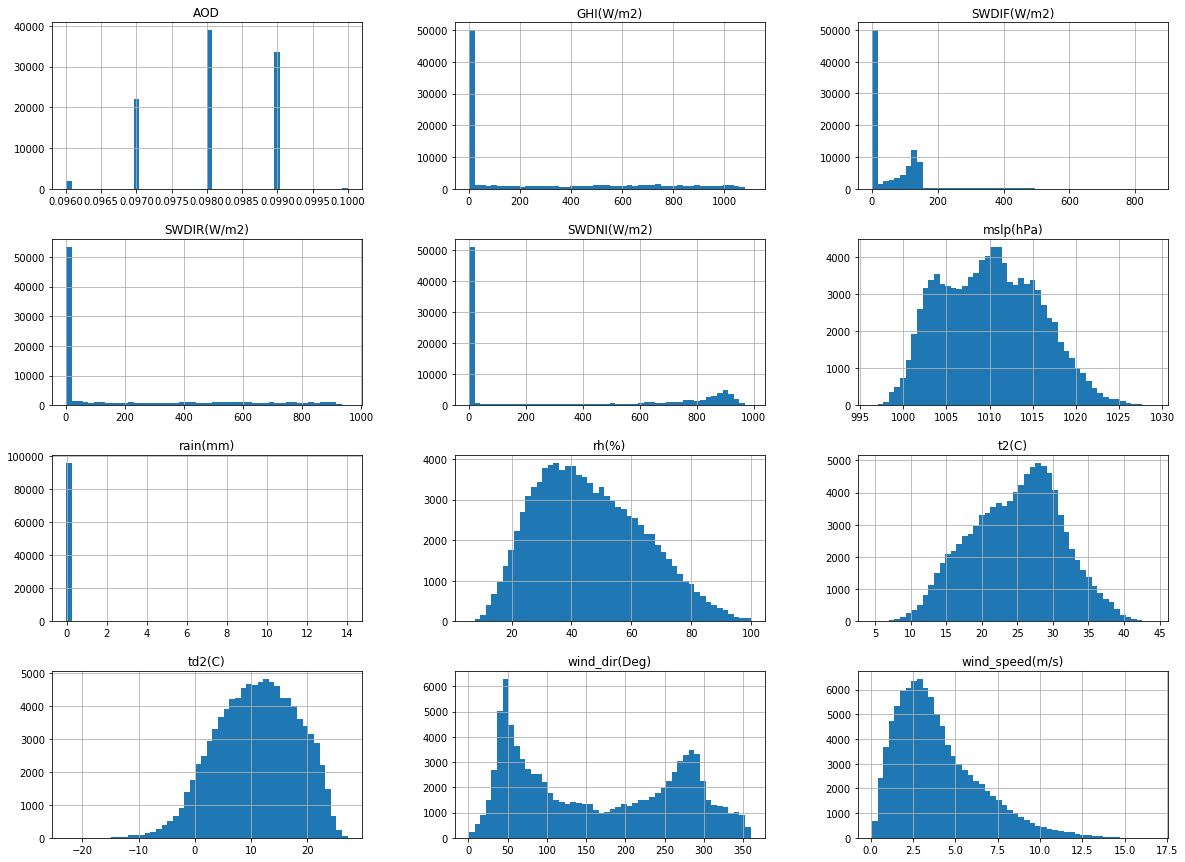
_ = neom_data.hist(bins=50, figsize=(20,15))
_hour = (neom_data.index
.hour
.rename("hour"))
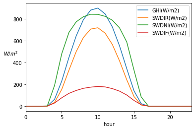
hourly_averages = (neom_data.groupby(_hour)
.mean())
fig, ax = plt.subplots(1, 1)
_targets = ["GHI(W/m2)", "SWDIR(W/m2)", "SWDNI(W/m2)", "SWDIF(W/m2)"]
(hourly_averages.loc[:, _targets]
.plot(ax=ax))
_ = ax.set_ylabel(r"$W/m^2$", rotation="horizontal")
months = (neom_data.index
.month
.rename("month"))
hours = (neom_data.index
.hour
.rename("hour"))
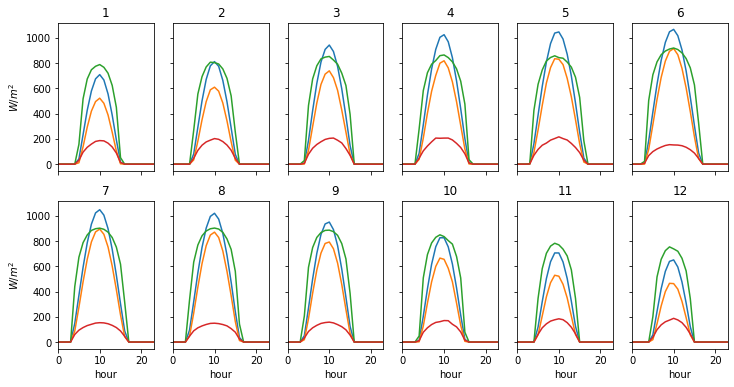
hourly_averages_by_month = (neom_data.groupby([months, hours])
.mean())
fig, axes = plt.subplots(2, 6, sharex=True, sharey=True, figsize=(12, 6))

for month in months.unique():
    if month <= 6:
        (hourly_averages_by_month.loc[month, _targets]
                                 .plot(ax=axes[0, month - 1], legend=False))
        _ = axes[0, month - 1].set_title(month)
    else:
        (hourly_averages_by_month.loc[month, _targets]
                                 .plot(ax=axes[1, month - 7], legend=False))
        _ = axes[1, month - 7].set_title(month)

    if month - 1 == 0:
        _ = axes[0, 0].set_ylabel(r"$W/m^2$")
    if month - 7 == 0:
        _ = axes[1, 0].set_ylabel(r"$W/m^2$")
Feature Engineering
neom_data.index.dayofweek.unique()
Int64Index([1, 2, 3, 4, 5, 6, 0], dtype='int64', name='Timestamp')
neom_data.index.weekofyear.unique()
Int64Index([ 1,  2,  3,  4,  5,  6,  7,  8,  9, 10, 11, 12, 13, 14, 15, 16, 17,
            18, 19, 20, 21, 22, 23, 24, 25, 26, 27, 28, 29, 30, 31, 32, 33, 34,
            35, 36, 37, 38, 39, 40, 41, 42, 43, 44, 45, 46, 47, 48, 49, 50, 51,
            52, 53],
           dtype='int64', name='Timestamp')
_dropped_cols = ["SWDIR(W/m2)", "SWDNI(W/m2)", "SWDIF(W/m2)"]

_year = (neom_data.index
                  .year)
_month = (neom_data.index
                   .month)
_week = (neom_data.index
                  .weekofyear)
_day = (neom_data.index
                 .dayofweek)
_hour = (neom_data.index
                  .hour)

features = (neom_data.drop(_dropped_cols, axis=1, inplace=False)
                     .assign(year=_year, month=_month, week=_week, day=_day, hour=_hour)
                     .groupby(["year", "month", "week", "day", "hour"])
                     .mean()
                     .unstack(level=["day", "hour"])
                     .reset_index(inplace=False)
                     .sort_index(axis=1)
                     .drop("year", axis=1, inplace=False)
                     .fillna(method="bfill", limit=2, inplace=False))
# want to predict the next 24 hours of "solar power"
efficiency_factor = 0.5

# square meters of solar cells required to generate 20 GW (231000 m2 will generate 7mW)
m2_of_solar_cells_required = 660000

target = (features.loc[:, ["GHI(W/m2)"]]
                  .mul(efficiency_factor)
                  .shift(-1)
                  .rename(columns={"GHI(W/m2)": "target(W/m2)"}))
target
| target(W/m2) | |||||||||||||||||||||
|---|---|---|---|---|---|---|---|---|---|---|---|---|---|---|---|---|---|---|---|---|---|
| day | 0 | ... | 6 | ||||||||||||||||||
| hour | 0 | 1 | 2 | 3 | 4 | 5 | 6 | 7 | 8 | 9 | ... | 14 | 15 | 16 | 17 | 18 | 19 | 20 | 21 | 22 | 23 |
| 0 | 0.0 | 0.0 | 0.0 | 0.0 | 0.0 | 15.4625 | 85.7540 | 199.4865 | 279.1695 | 328.9370 | ... | 103.1305 | 4.8625 | 0.0 | 0.0 | 0.0 | 0.0 | 0.0 | 0.0 | 0.0 | 0.0 |
| 1 | 0.0 | 0.0 | 0.0 | 0.0 | 0.0 | 22.0325 | 128.9640 | 233.4150 | 315.5565 | 366.3655 | ... | 74.5395 | 7.7545 | 0.0 | 0.0 | 0.0 | 0.0 | 0.0 | 0.0 | 0.0 | 0.0 |
| 2 | 0.0 | 0.0 | 0.0 | 0.0 | 0.0 | 9.2310 | 71.1300 | 97.3875 | 65.3585 | 102.5280 | ... | 119.8195 | 17.9220 | 0.0 | 0.0 | 0.0 | 0.0 | 0.0 | 0.0 | 0.0 | 0.0 |
| 3 | 0.0 | 0.0 | 0.0 | 0.0 | 0.0 | 24.6660 | 129.5175 | 233.2570 | 316.0465 | 368.8395 | ... | 136.2110 | 27.3505 | 0.0 | 0.0 | 0.0 | 0.0 | 0.0 | 0.0 | 0.0 | 0.0 |
| 4 | 0.0 | 0.0 | 0.0 | 0.0 | 0.0 | 30.6040 | 140.9780 | 248.4170 | 334.1340 | 388.3575 | ... | 136.2110 | 27.3505 | 0.0 | 0.0 | 0.0 | 0.0 | 0.0 | 0.0 | 0.0 | 0.0 |
| ... | ... | ... | ... | ... | ... | ... | ... | ... | ... | ... | ... | ... | ... | ... | ... | ... | ... | ... | ... | ... | ... |
| 683 | 0.0 | 0.0 | 0.0 | 0.0 | 0.0 | 26.1075 | 98.4485 | 163.9655 | 226.5005 | 224.1960 | ... | 59.4640 | 0.0000 | 0.0 | 0.0 | 0.0 | 0.0 | 0.0 | 0.0 | 0.0 | 0.0 |
| 684 | 0.0 | 0.0 | 0.0 | 0.0 | 0.0 | 33.3755 | 130.9790 | 222.7225 | 291.9230 | 331.0915 | ... | 46.6540 | 0.0000 | 0.0 | 0.0 | 0.0 | 0.0 | 0.0 | 0.0 | 0.0 | 0.0 |
| 685 | 0.0 | 0.0 | 0.0 | 0.0 | 0.0 | 21.9080 | 122.6125 | 214.2285 | 285.8000 | 328.2050 | ... | 68.8560 | 0.0000 | 0.0 | 0.0 | 0.0 | 0.0 | 0.0 | 0.0 | 0.0 | 0.0 |
| 686 | 0.0 | 0.0 | 0.0 | 0.0 | 0.0 | 21.6690 | 114.3185 | 214.0540 | 286.2330 | 335.3290 | ... | 75.8040 | 0.0000 | 0.0 | 0.0 | 0.0 | 0.0 | 0.0 | 0.0 | 0.0 | 0.0 |
| 687 | NaN | NaN | NaN | NaN | NaN | NaN | NaN | NaN | NaN | NaN | ... | NaN | NaN | NaN | NaN | NaN | NaN | NaN | NaN | NaN | NaN |
688 rows × 168 columns
input_data = (features.join(target)
                      .dropna(how="any", inplace=False)
                      .sort_index(axis=1))
input_data
| AOD | ... | wind_speed(m/s) | |||||||||||||||||||
|---|---|---|---|---|---|---|---|---|---|---|---|---|---|---|---|---|---|---|---|---|---|
| day | 0 | ... | 6 | ||||||||||||||||||
| hour | 0 | 1 | 2 | 3 | 4 | 5 | 6 | 7 | 8 | 9 | ... | 14 | 15 | 16 | 17 | 18 | 19 | 20 | 21 | 22 | 23 |
| 0 | 0.097 | 0.097 | 0.097 | 0.097 | 0.097 | 0.097 | 0.097 | 0.097 | 0.097 | 0.097 | ... | 8.923 | 8.388 | 9.168 | 8.932 | 8.275 | 7.644 | 7.218 | 7.145 | 7.254 | 7.519 |
| 1 | 0.097 | 0.097 | 0.097 | 0.097 | 0.097 | 0.097 | 0.097 | 0.097 | 0.097 | 0.097 | ... | 9.678 | 8.897 | 9.666 | 10.197 | 10.668 | 11.314 | 11.842 | 11.067 | 10.485 | 10.239 |
| 2 | 0.097 | 0.097 | 0.097 | 0.097 | 0.097 | 0.097 | 0.097 | 0.097 | 0.096 | 0.096 | ... | 2.601 | 1.350 | 0.610 | 0.728 | 0.907 | 3.140 | 2.474 | 2.689 | 1.970 | 2.567 |
| 3 | 0.097 | 0.097 | 0.097 | 0.097 | 0.097 | 0.097 | 0.097 | 0.097 | 0.097 | 0.097 | ... | 4.836 | 4.340 | 3.016 | 2.484 | 2.084 | 2.861 | 4.209 | 3.804 | 3.431 | 3.677 |
| 4 | 0.097 | 0.097 | 0.097 | 0.097 | 0.097 | 0.097 | 0.097 | 0.097 | 0.097 | 0.097 | ... | 6.908 | 5.829 | 6.632 | 8.176 | 8.604 | 8.674 | 8.467 | 7.488 | 6.633 | 5.573 |
| ... | ... | ... | ... | ... | ... | ... | ... | ... | ... | ... | ... | ... | ... | ... | ... | ... | ... | ... | ... | ... | ... |
| 682 | 0.097 | 0.097 | 0.097 | 0.097 | 0.097 | 0.097 | 0.097 | 0.097 | 0.097 | 0.097 | ... | 2.619 | 1.129 | 1.292 | 1.148 | 0.652 | 2.440 | 2.516 | 2.264 | 1.588 | 1.944 |
| 683 | 0.098 | 0.098 | 0.098 | 0.098 | 0.098 | 0.098 | 0.098 | 0.098 | 0.098 | 0.098 | ... | 2.619 | 1.129 | 1.292 | 1.148 | 0.652 | 2.440 | 2.516 | 2.264 | 1.588 | 1.944 |
| 684 | 0.098 | 0.098 | 0.098 | 0.098 | 0.098 | 0.098 | 0.098 | 0.098 | 0.098 | 0.098 | ... | 3.986 | 3.138 | 2.724 | 2.075 | 2.061 | 3.872 | 3.611 | 3.181 | 2.318 | 1.720 |
| 685 | 0.097 | 0.097 | 0.097 | 0.097 | 0.097 | 0.097 | 0.097 | 0.097 | 0.097 | 0.097 | ... | 2.699 | 1.082 | 1.608 | 2.728 | 2.096 | 0.757 | 0.874 | 2.458 | 3.756 | 3.466 |
| 686 | 0.097 | 0.097 | 0.097 | 0.097 | 0.097 | 0.097 | 0.097 | 0.097 | 0.097 | 0.097 | ... | 1.157 | 1.639 | 4.840 | 5.091 | 4.948 | 5.264 | 5.263 | 4.680 | 4.376 | 3.756 |
687 rows × 1682 columns
Train, Test Split
# use first 10 years for training data...
training_data = input_data.loc[:10 * 53]

# ...next two years for validation data...
validation_data = input_data.loc[10 * 53 + 1:12 * 53]

# ...and final year for testing data!
testing_data = input_data.loc[12 * 53 + 1:]
training_data.shape
(531, 1682)
validation_data.shape
(106, 1682)
testing_data.shape
(50, 1682)
Preprocessing the training and validation data
def preprocess_features(df: pd.DataFrame) -> pd.DataFrame:
    _numeric_features = ["GHI(W/m2)",
                         "mslp(hPa)",
                         "rain(mm)",
                         "rh(%)",
                         "t2(C)",
                         "td2(C)",
                         "wind_dir(Deg)",
                         "wind_speed(m/s)"]

    _ordinal_features = ["AOD",
                         "day",
                         "month",
                         "year"]

    standard_scalar = preprocessing.StandardScaler()
    Z0 = standard_scalar.fit_transform(df.loc[:, _numeric_features])

    ordinal_encoder = preprocessing.OrdinalEncoder()
    Z1 = ordinal_encoder.fit_transform(df.loc[:, _ordinal_features])
    transformed_features = np.hstack((Z0, Z1))

    return transformed_features
training_features = training_data.drop("target(W/m2)", axis=1, inplace=False)
training_target = training_data.loc[:, ["target(W/m2)"]]
transformed_training_features = preprocess_features(training_features)

validation_features = validation_data.drop("target(W/m2)", axis=1, inplace=False)
validation_target = validation_data.loc[:, ["target(W/m2)"]]
transformed_validation_features = preprocess_features(validation_features)
Find a few models that seem to work well
Linear Regression
# training a liner regression model
linear_regression = linear_model.LinearRegression()
linear_regression.fit(transformed_training_features, training_target)
LinearRegression(copy_X=True, fit_intercept=True, n_jobs=None, normalize=False)
# measure training error
_predictions = linear_regression.predict(transformed_training_features)
np.sqrt(metrics.mean_squared_error(training_target, _predictions))
3.5984482821003514e-13
# measure training error
_predictions = linear_regression.predict(transformed_validation_features)
np.sqrt(metrics.mean_squared_error(validation_target, _predictions))
41.65348268671971
# user requests forecast for some week
user_forecast_request = transformed_validation_features[[-1], :]
user_forecast_response = linear_regression.predict(user_forecast_request)[0]
actual_values_response = validation_target.values[[-1], :][0]

# this would be rendered in Tableau!
plt.plot(user_forecast_response, label="predicted")
plt.plot(actual_values_response, label="actual")
plt.legend()
plt.title("Weekly forecast")
plt.ylabel("Solar Power (W/m2)")
plt.xlabel("Hour")
Text(0.5, 0, 'Hour')
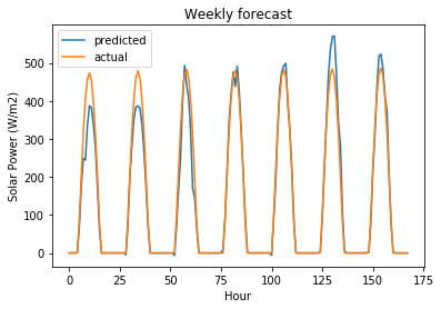
Linear regression is overfitting!
MultiTask ElasticNet Regression
# training a multi-task elastic net model
_prng = np.random.RandomState(42)
elastic_net = linear_model.MultiTaskElasticNet(random_state=_prng)
elastic_net.fit(transformed_training_features, training_target)
/Users/pughdr/Research/junctionx-kaust-2019/env/lib/python3.6/site-packages/sklearn/linear_model/coordinate_descent.py:1803: ConvergenceWarning: Objective did not converge. You might want to increase the number of iterations. Duality gap: 3211704.2181589045, tolerance: 24372.85566059234
  check_random_state(self.random_state), random)


MultiTaskElasticNet(alpha=1.0, copy_X=True, fit_intercept=True, l1_ratio=0.5,
                    max_iter=1000, normalize=False,
                    random_state=<mtrand.RandomState object at 0x1a2be47f30>,
                    selection='cyclic', tol=0.0001, warm_start=False)
# measure training error
_predictions = elastic_net.predict(transformed_training_features)
np.sqrt(metrics.mean_squared_error(training_target, _predictions))
12.62446635442459
# measure validation error
_predictions = elastic_net.predict(transformed_validation_features)
np.sqrt(metrics.mean_squared_error(validation_target, _predictions))
21.755388481701576
user_forecast_request = transformed_validation_features[[-1], :]
user_forecast_response = elastic_net.predict(user_forecast_request)[0]
actual_values_response = validation_target.values[[-1], :][0]

# this would be rendered in Tableau!
plt.plot(user_forecast_response, label="predicted")
plt.plot(actual_values_response, label="actual")
plt.legend()
plt.title("Weekly forecast")
plt.ylabel("Solar Power (W/m2)")
plt.xlabel("Hour")
Text(0.5, 0, 'Hour')
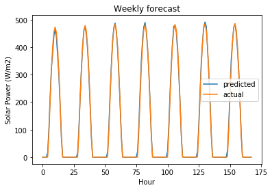
MultiTask ElasticNet is still underfitting with default values but does significantly better than plain linear regression.
MultiTask Lasso Regression
# training a multi-task lasso model
_prng = np.random.RandomState(42)
lasso_regression = linear_model.MultiTaskLasso(random_state=_prng)
lasso_regression.fit(transformed_training_features, training_target)
/Users/pughdr/Research/junctionx-kaust-2019/env/lib/python3.6/site-packages/sklearn/linear_model/coordinate_descent.py:1803: ConvergenceWarning: Objective did not converge. You might want to increase the number of iterations. Duality gap: 344470.44411674794, tolerance: 24372.85566059234
  check_random_state(self.random_state), random)


MultiTaskLasso(alpha=1.0, copy_X=True, fit_intercept=True, max_iter=1000,
               normalize=False,
               random_state=<mtrand.RandomState object at 0x1a2cb81c18>,
               selection='cyclic', tol=0.0001, warm_start=False)
# measure training error
_predictions = lasso_regression.predict(transformed_training_features)
np.sqrt(metrics.mean_squared_error(training_target, _predictions))
9.142156744519834
# measure validation error
_predictions = lasso_regression.predict(transformed_validation_features)
np.sqrt(metrics.mean_squared_error(validation_target, _predictions))
25.11003195102284
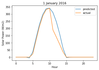
user_forecast_request = transformed_validation_features[[-1], :]
user_forecast_response = lasso_regression.predict(user_forecast_request)[0]
actual_values_response = validation_target.values[[-1], :][0]

# this would be rendered in Tableau!
plt.plot(user_forecast_response, label="predicted")
plt.plot(actual_values_response, label="actual")
plt.legend()
plt.title("1 January 2016")
plt.ylabel("Solar Power (W/m2)")
plt.xlabel("Hour")
Text(0.5, 0, 'Hour')
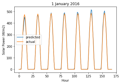
Lasso Regression is over-fitting.
Random Forest Regression
_prng = np.random.RandomState(42)
random_forest_regressor = ensemble.RandomForestRegressor(n_estimators=100, random_state=_prng, n_jobs=2)
random_forest_regressor.fit(transformed_training_features, training_target)
RandomForestRegressor(bootstrap=True, criterion='mse', max_depth=None,
                      max_features='auto', max_leaf_nodes=None,
                      min_impurity_decrease=0.0, min_impurity_split=None,
                      min_samples_leaf=1, min_samples_split=2,
                      min_weight_fraction_leaf=0.0, n_estimators=100, n_jobs=2,
                      oob_score=False,
                      random_state=<mtrand.RandomState object at 0x1a2cc2bbd0>,
                      verbose=0, warm_start=False)
# measure training error
_predictions = random_forest_regressor.predict(transformed_training_features)
np.sqrt(metrics.mean_squared_error(training_target, _predictions))
7.011236706071975
# measure validation error
_predictions = random_forest_regressor.predict(transformed_validation_features)
np.sqrt(metrics.mean_squared_error(validation_target, _predictions))
19.32772745697949
user_forecast_request = transformed_validation_features[[-1], :]
user_forecast_response = random_forest_regressor.predict(user_forecast_request)[0]
actual_values_response = validation_target.values[[-1], :][0]

# this would be rendered in Tableau!
plt.plot(user_forecast_response, label="predicted")
plt.plot(actual_values_response, label="actual")
plt.legend()
plt.title("Weekly Forecast")
plt.ylabel("Solar Power (W/m2)")
plt.xlabel("Hour")
Text(0.5, 0, 'Hour')
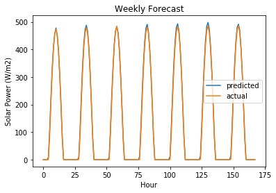
Random Forest with default parameters is over-fitting and needs to be regularized.
Tuning hyper-parameters
from scipy import stats
MultiTask ElasticNet Regression
_prng = np.random.RandomState(42)

_param_distributions = {
    "l1_ratio": stats.uniform(),
    "alpha": stats.lognorm(s=1),
}

elastic_net_randomized_search = model_selection.RandomizedSearchCV(
    elastic_net,
    param_distributions=_param_distributions,
    scoring="neg_mean_squared_error",
    random_state=_prng,
    n_iter=10,
    cv=8,
    n_jobs=2,
    verbose=10
)

elastic_net_randomized_search.fit(transformed_training_features, training_target)
Fitting 8 folds for each of 10 candidates, totalling 80 fits


[Parallel(n_jobs=2)]: Using backend LokyBackend with 2 concurrent workers.
[Parallel(n_jobs=2)]: Done   1 tasks      | elapsed:  2.8min
[Parallel(n_jobs=2)]: Done   4 tasks      | elapsed:  5.5min


---------------------------------------------------------------------------

KeyboardInterrupt                         Traceback (most recent call last)

<ipython-input-94-47f8877f33d1> in <module>
     17 )
     18
---> 19 elastic_net_randomized_search.fit(transformed_training_features, training_target)


~/Research/junctionx-kaust-2019/env/lib/python3.6/site-packages/sklearn/model_selection/_search.py in fit(self, X, y, groups, **fit_params)
    685                 return results
    686
--> 687             self._run_search(evaluate_candidates)
    688
    689         # For multi-metric evaluation, store the best_index_, best_params_ and


~/Research/junctionx-kaust-2019/env/lib/python3.6/site-packages/sklearn/model_selection/_search.py in _run_search(self, evaluate_candidates)
   1466         evaluate_candidates(ParameterSampler(
   1467             self.param_distributions, self.n_iter,
-> 1468             random_state=self.random_state))


~/Research/junctionx-kaust-2019/env/lib/python3.6/site-packages/sklearn/model_selection/_search.py in evaluate_candidates(candidate_params)
    664                                for parameters, (train, test)
    665                                in product(candidate_params,
--> 666                                           cv.split(X, y, groups)))
    667
    668                 if len(out) < 1:


~/Research/junctionx-kaust-2019/env/lib/python3.6/site-packages/joblib/parallel.py in __call__(self, iterable)
    932
    933             with self._backend.retrieval_context():
--> 934                 self.retrieve()
    935             # Make sure that we get a last message telling us we are done
    936             elapsed_time = time.time() - self._start_time


~/Research/junctionx-kaust-2019/env/lib/python3.6/site-packages/joblib/parallel.py in retrieve(self)
    831             try:
    832                 if getattr(self._backend, 'supports_timeout', False):
--> 833                     self._output.extend(job.get(timeout=self.timeout))
    834                 else:
    835                     self._output.extend(job.get())


~/Research/junctionx-kaust-2019/env/lib/python3.6/site-packages/joblib/_parallel_backends.py in wrap_future_result(future, timeout)
    519         AsyncResults.get from multiprocessing."""
    520         try:
--> 521             return future.result(timeout=timeout)
    522         except LokyTimeoutError:
    523             raise TimeoutError()


~/Research/junctionx-kaust-2019/env/lib/python3.6/concurrent/futures/_base.py in result(self, timeout)
    425                 return self.__get_result()
    426
--> 427             self._condition.wait(timeout)
    428
    429             if self._state in [CANCELLED, CANCELLED_AND_NOTIFIED]:


~/Research/junctionx-kaust-2019/env/lib/python3.6/threading.py in wait(self, timeout)
    293         try:    # restore state no matter what (e.g., KeyboardInterrupt)
    294             if timeout is None:
--> 295                 waiter.acquire()
    296                 gotit = True
    297             else:


KeyboardInterrupt:
_ = joblib.dump(elastic_net_randomized_search.best_estimator_,
                "../models/weekly/tuned-elasticnet-regression-model.pkl")
elastic_net_randomized_search.best_estimator_
MultiTaskElasticNet(alpha=2.154232968599504, copy_X=True, fit_intercept=True,
                    l1_ratio=0.9699098521619943, max_iter=1000, normalize=False,
                    random_state=<mtrand.RandomState object at 0x1a48e31558>,
                    selection='cyclic', tol=0.0001, warm_start=False)
(-elastic_net_randomized_search.best_score_)**0.5
18.355092813714375
user_forecast_request = transformed_validation_features[[-1], :]
user_forecast_response = elastic_net_randomized_search.predict(user_forecast_request)[0]
actual_values_response = validation_target.values[[-1], :][0]

# this would be rendered in Tableau!
plt.plot(user_forecast_response, label="predicted")
plt.plot(actual_values_response, label="actual")
plt.legend()
plt.title("Typical weekyl forecast")
plt.ylabel("Solar Power (W/m2)")
plt.xlabel("Hour")
Text(0.5, 0, 'Hour')
MultiTask Lasso Regression
_prng = np.random.RandomState(42)

_param_distributions = {
    "alpha": stats.lognorm(s=1),
}

lasso_regression_randomized_search = model_selection.RandomizedSearchCV(
    lasso_regression,
    param_distributions=_param_distributions,
    scoring="neg_mean_squared_error",
    random_state=_prng,
    n_iter=10,
    cv=8,
    n_jobs=2,
    verbose=10
)

lasso_regression_randomized_search.fit(transformed_training_features, training_target)
Fitting 8 folds for each of 10 candidates, totalling 80 fits


[Parallel(n_jobs=2)]: Using backend LokyBackend with 2 concurrent workers.
[Parallel(n_jobs=2)]: Done   1 tasks      | elapsed:    7.0s
[Parallel(n_jobs=2)]: Done   4 tasks      | elapsed:    9.4s
[Parallel(n_jobs=2)]: Done   9 tasks      | elapsed:   16.5s
[Parallel(n_jobs=2)]: Done  14 tasks      | elapsed:   22.5s
[Parallel(n_jobs=2)]: Done  21 tasks      | elapsed:   30.3s
[Parallel(n_jobs=2)]: Done  28 tasks      | elapsed:   38.4s
[Parallel(n_jobs=2)]: Done  37 tasks      | elapsed:   48.6s
[Parallel(n_jobs=2)]: Done  46 tasks      | elapsed:  1.0min
[Parallel(n_jobs=2)]: Done  57 tasks      | elapsed:  1.2min
[Parallel(n_jobs=2)]: Done  68 tasks      | elapsed:  1.5min
[Parallel(n_jobs=2)]: Done  80 out of  80 | elapsed:  1.8min finished


RandomizedSearchCV(cv=8, error_score='raise-deprecating',
                   estimator=MultiTaskLasso(alpha=1.0, copy_X=True,
                                            fit_intercept=True, max_iter=1000,
                                            normalize=False,
                                            random_state=<mtrand.RandomState object at 0x1a649d5870>,
                                            selection='cyclic', tol=0.0001,
                                            warm_start=False),
                   iid='warn', n_iter=10, n_jobs=2,
                   param_distributions={'alpha': <scipy.stats._distn_infrastructure.rv_frozen object at 0x1a7af2b470>},
                   pre_dispatch='2*n_jobs',
                   random_state=<mtrand.RandomState object at 0x1a69473438>,
                   refit=True, return_train_score=False,
                   scoring='neg_mean_squared_error', verbose=10)
_ = joblib.dump(lasso_regression_randomized_search.best_estimator_,
                "../models/weekly/tuned-lasso-regression-model.pkl")
(-lasso_regression_randomized_search.best_score_)**0.5
17.956920842745834
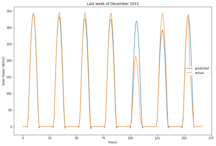
user_forecast_request = transformed_validation_features[-7:, :]
user_forecast_response = lasso_regression_randomized_search.predict(user_forecast_request)
actual_values_response = validation_target.values[-7:, :]

# this would be rendered in Tableau!
fig, ax = plt.subplots(1, 1, figsize=(12, 8))
ax.plot(user_forecast_response.flatten(), label="predicted")
ax.plot(actual_values_response.flatten(), label="actual")
ax.legend()
ax.set_title("Last week of December 2015")
ax.set_ylabel("Solar Power (W/m2)")
ax.set_xlabel("Hours")
Text(0.5, 0, 'Hours')
Random Forest Regressor
_prng = np.random.RandomState(42)

_param_distributions = {
    "n_estimators": stats.geom(p=0.01),
     "min_samples_split": stats.beta(a=1, b=99),
     "min_samples_leaf": stats.beta(a=1, b=999),
}

_cv = model_selection.TimeSeriesSplit(max_train_size=None, n_splits=5)

random_forest_randomized_search = model_selection.RandomizedSearchCV(
    random_forest_regressor,
    param_distributions=_param_distributions,
    scoring="neg_mean_squared_error",
    random_state=_prng,
    n_iter=10,
    cv=3,
    n_jobs=2,
    verbose=10
)

random_forest_randomized_search.fit(transformed_training_features, training_target)
Fitting 3 folds for each of 10 candidates, totalling 30 fits


[Parallel(n_jobs=2)]: Using backend LokyBackend with 2 concurrent workers.
[Parallel(n_jobs=2)]: Done   1 tasks      | elapsed:  1.2min
[Parallel(n_jobs=2)]: Done   4 tasks      | elapsed:  2.3min
[Parallel(n_jobs=2)]: Done   9 tasks      | elapsed: 14.0min
[Parallel(n_jobs=2)]: Done  14 tasks      | elapsed: 14.8min
[Parallel(n_jobs=2)]: Done  21 tasks      | elapsed: 15.4min
[Parallel(n_jobs=2)]: Done  30 out of  30 | elapsed: 18.4min finished


RandomizedSearchCV(cv=3, error_score='raise-deprecating',
                   estimator=RandomForestRegressor(bootstrap=True,
                                                   criterion='mse',
                                                   max_depth=None,
                                                   max_features='auto',
                                                   max_leaf_nodes=None,
                                                   min_impurity_decrease=0.0,
                                                   min_impurity_split=None,
                                                   min_samples_leaf=1,
                                                   min_samples_split=2,
                                                   min_weight_fraction_leaf=0.0,
                                                   n_estimators=100, n_jobs=2,
                                                   oob_score=False,
                                                   random_state=<mt...
                   param_distributions={'min_samples_leaf': <scipy.stats._distn_infrastructure.rv_frozen object at 0x1a28d373c8>,
                                        'min_samples_split': <scipy.stats._distn_infrastructure.rv_frozen object at 0x1a28d375f8>,
                                        'n_estimators': <scipy.stats._distn_infrastructure.rv_frozen object at 0x1a28d28630>},
                   pre_dispatch='2*n_jobs',
                   random_state=<mtrand.RandomState object at 0x1a2886e828>,
                   refit=True, return_train_score=False,
                   scoring='neg_mean_squared_error', verbose=10)
_ = joblib.dump(random_forest_randomized_search.best_estimator_,
                "../models/weekly/tuned-random-forest-regression-model.pkl")
random_forest_randomized_search.best_estimator_
RandomForestRegressor(bootstrap=True, criterion='mse', max_depth=None,
                      max_features='auto', max_leaf_nodes=None,
                      min_impurity_decrease=0.0, min_impurity_split=None,
                      min_samples_leaf=0.001249828663231378,
                      min_samples_split=0.0019415164208264953,
                      min_weight_fraction_leaf=0.0, n_estimators=75, n_jobs=2,
                      oob_score=False,
                      random_state=<mtrand.RandomState object at 0x1a292509d8>,
                      verbose=0, warm_start=False)
(-random_forest_randomized_search.best_score_)**0.5
19.002834611158974
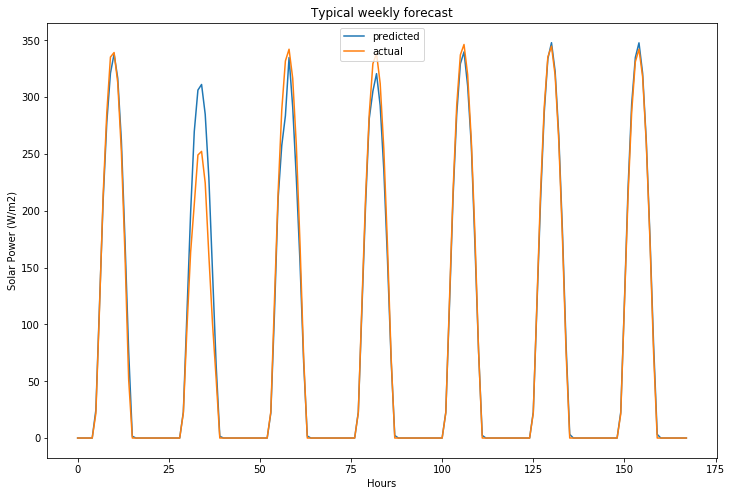
# user requests forecast for 1 January 2016 which we predict using data from 31 December 2015!
user_forecast_request = transformed_validation_features[[-1], :]
user_forecast_response = random_forest_randomized_search.predict(user_forecast_request)[0]
actual_values_response = validation_target.values[[-1], :][0]

# this would be rendered in Tableau!
plt.plot(user_forecast_response, label="predicted")
plt.plot(actual_values_response, label="actual")
plt.legend()
plt.title("Typical weekly forecast")
plt.ylabel("Solar Power (W/m2)")
plt.xlabel("Hour")
Assess model performance on testing data
testing_features = testing_data.drop("target(W/m2)", axis=1, inplace=False)
testing_target = testing_data.loc[:, ["target(W/m2)"]]
transformed_testing_features = preprocess_features(testing_features)
elastic_net_predictions = elastic_net_randomized_search.predict(transformed_testing_features)
np.sqrt(metrics.mean_squared_error(testing_target, elastic_net_predictions))
19.76022744338562
lasso_regression_predictions = lasso_regression_randomized_search.predict(transformed_testing_features)
np.sqrt(metrics.mean_squared_error(testing_target, lasso_regression_predictions))
19.73446980783998
# random forest wins!
random_forest_predictions = random_forest_randomized_search.predict(transformed_testing_features)
np.sqrt(metrics.mean_squared_error(testing_target, random_forest_predictions))
19.826312994581507
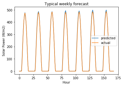
# user requests forecast for last week of 2018
user_forecast_request = transformed_testing_features[[-1], :]
user_forecast_response = random_forest_randomized_search.predict(user_forecast_request)[0]
actual_values_response = testing_target.values[[-1], :][0]

# this would be rendered in Tableau!
fig, ax = plt.subplots(1, 1, figsize=(12, 8))
ax.plot(user_forecast_response.flatten(), label="predicted")
ax.plot(actual_values_response.flatten(), label="actual")
ax.legend()
ax.set_title("Typical weekly forecast")
ax.set_ylabel("Solar Power (W/m2)")
ax.set_xlabel("Hours")
plt.savefig("../results/img/typical-weekly-actual-vs-predicted-solar-power.png")
# combine the training and validtion data
combined_training_features = pd.concat([training_features, validation_features])
transformed_combined_training_features = preprocess_features(combined_training_features)
combined_training_target = pd.concat([training_target, validation_target])

# tune a random forest regressor using CV ro avoid overfitting
_prng = np.random.RandomState(42)

_param_distributions = {
    "n_estimators": stats.geom(p=0.01),
     "min_samples_split": stats.beta(a=1, b=99),
     "min_samples_leaf": stats.beta(a=1, b=999),
}

tuned_random_forest_regressor = model_selection.RandomizedSearchCV(
    ensemble.RandomForestRegressor(n_estimators=100, random_state=_prng),
    param_distributions=_param_distributions,
    scoring="neg_mean_squared_error",
    random_state=_prng,
    n_iter=10,
    cv=5,
    n_jobs=2,
    verbose=10
)

tuned_random_forest_regressor.fit(combined_training_features, combined_training_target)
Fitting 5 folds for each of 10 candidates, totalling 50 fits


[Parallel(n_jobs=2)]: Using backend LokyBackend with 2 concurrent workers.
[Parallel(n_jobs=2)]: Done   1 tasks      | elapsed:  2.5min
[Parallel(n_jobs=2)]: Done   4 tasks      | elapsed:  4.9min
[Parallel(n_jobs=2)]: Done   9 tasks      | elapsed: 10.5min
[Parallel(n_jobs=2)]: Done  14 tasks      | elapsed: 14.2min
[Parallel(n_jobs=2)]: Done  21 tasks      | elapsed: 16.4min
[Parallel(n_jobs=2)]: Done  28 tasks      | elapsed: 17.9min
[Parallel(n_jobs=2)]: Done  37 tasks      | elapsed: 20.3min
[Parallel(n_jobs=2)]: Done  46 tasks      | elapsed: 26.2min
[Parallel(n_jobs=2)]: Done  50 out of  50 | elapsed: 28.3min finished
/Users/pughdr/Research/junctionx-kaust-2019/env/lib/python3.6/site-packages/sklearn/model_selection/_search.py:813: DeprecationWarning: The default of the `iid` parameter will change from True to False in version 0.22 and will be removed in 0.24. This will change numeric results when test-set sizes are unequal.
  DeprecationWarning)


RandomizedSearchCV(cv=5, error_score='raise-deprecating',
                   estimator=RandomForestRegressor(bootstrap=True,
                                                   criterion='mse',
                                                   max_depth=None,
                                                   max_features='auto',
                                                   max_leaf_nodes=None,
                                                   min_impurity_decrease=0.0,
                                                   min_impurity_split=None,
                                                   min_samples_leaf=1,
                                                   min_samples_split=2,
                                                   min_weight_fraction_leaf=0.0,
                                                   n_estimators=100,
                                                   n_jobs=None, oob_score=False,
                                                   random_state=...
                   param_distributions={'min_samples_leaf': <scipy.stats._distn_infrastructure.rv_frozen object at 0x1a32bef860>,
                                        'min_samples_split': <scipy.stats._distn_infrastructure.rv_frozen object at 0x1a32bef198>,
                                        'n_estimators': <scipy.stats._distn_infrastructure.rv_frozen object at 0x1a32bef7f0>},
                   pre_dispatch='2*n_jobs',
                   random_state=<mtrand.RandomState object at 0x1a2cc608b8>,
                   refit=True, return_train_score=False,
                   scoring='neg_mean_squared_error', verbose=10)
tuned_random_forest_regressor.best_estimator_
RandomForestRegressor(bootstrap=True, criterion='mse', max_depth=None,
                      max_features='auto', max_leaf_nodes=None,
                      min_impurity_decrease=0.0, min_impurity_split=None,
                      min_samples_leaf=0.0004129137216396695,
                      min_samples_split=0.004789233605970227,
                      min_weight_fraction_leaf=0.0, n_estimators=78,
                      n_jobs=None, oob_score=False,
                      random_state=<mtrand.RandomState object at 0x1a32c13948>,
                      verbose=0, warm_start=False)
(-tuned_random_forest_regressor.best_score_)**0.5
18.785573993005393
# user requests forecast for last week of 2018
user_forecast_request = transformed_testing_features[[-1], :]
user_forecast_response = random_forest_randomized_search.predict(user_forecast_request)[0]
actual_values_response = testing_target.values[[-1], :][0]

# this would be rendered in Tableau!
fig, ax = plt.subplots(1, 1, figsize=(12, 8))
ax.plot(user_forecast_response.flatten(), label="predicted")
ax.plot(actual_values_response.flatten(), label="actual")
ax.legend()
ax.set_title("Typical weekly forecast")
ax.set_ylabel("Solar Power (W/m2)")
ax.set_xlabel("Hours")
plt.savefig("../results/img/typical-weekly-actual-vs-predicted-solar-power.png")

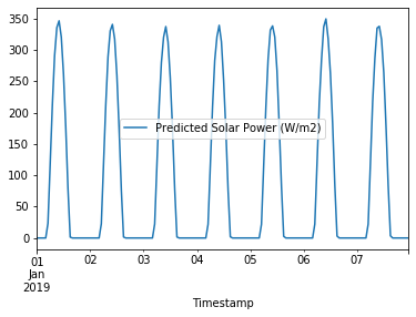
Forecasting the future of solar power at NEOM
Once the model is trained, the model can generate a new forecast for next week’s solar power generation. Once actual values of solar power generation are observed, model can be automatically re-trained and improved. Model can be retrained with weekly, monthly forecast horizons if longer forecasts are required.
incoming_features = features.loc[[687]]
new_predictions = tuned_random_forest_regressor.predict(incoming_features)[0]
solar_power_forecast = (pd.DataFrame.from_dict({"Timestamp": pd.date_range(start="2019-01-01", end="2019-01-07 23:00:00", freq='H'),
                                                "Predicted Solar Power (W/m2)": new_predictions})
                          .set_index("Timestamp", inplace=False))
_ = solar_power_forecast.plot()