This is the jupyter notebook from our JunctionX kaust hackaton (24h forecast), source is here
import matplotlib.pyplot as plt
import numpy as np
import pandas as pd
from sklearn import linear_model, ensemble, metrics, model_selection, preprocessing
import joblib
%matplotlib inline
Predicting Solar Power Output at NEOM
neom_data = (pd.read_csv("../data/raw/neom-data.csv", parse_dates=[0])
               .rename(columns={"Unnamed: 0": "Timestamp"})
               .set_index("Timestamp", drop=True, inplace=False))
neom_data.info()
<class 'pandas.core.frame.DataFrame'>
DatetimeIndex: 96432 entries, 2008-01-01 00:00:00 to 2018-12-31 23:00:00
Data columns (total 12 columns):
mslp(hPa)          96432 non-null float64
t2(C)              96432 non-null float64
td2(C)             96432 non-null float64
wind_speed(m/s)    96432 non-null float64
wind_dir(Deg)      96432 non-null float64
rh(%)              96432 non-null float64
GHI(W/m2)          96432 non-null float64
SWDIR(W/m2)        96432 non-null float64
SWDNI(W/m2)        96432 non-null float64
SWDIF(W/m2)        96432 non-null float64
rain(mm)           96432 non-null float64
AOD                96432 non-null float64
dtypes: float64(12)
memory usage: 9.6 MB
neom_data.head()
| mslp(hPa) | t2(C) | td2(C) | wind_speed(m/s) | wind_dir(Deg) | rh(%) | GHI(W/m2) | SWDIR(W/m2) | SWDNI(W/m2) | SWDIF(W/m2) | rain(mm) | AOD | |
|---|---|---|---|---|---|---|---|---|---|---|---|---|
| Timestamp | ||||||||||||
| 2008-01-01 00:00:00 | 1012.751 | 14.887 | 2.606 | 2.669 | 105.078 | 43.686 | 0.0 | 0.0 | 0.0 | 0.0 | 0.0 | 0.098 |
| 2008-01-01 01:00:00 | 1012.917 | 14.429 | 3.363 | 2.667 | 106.699 | 47.442 | 0.0 | 0.0 | 0.0 | 0.0 | 0.0 | 0.098 |
| 2008-01-01 02:00:00 | 1012.966 | 14.580 | 3.778 | 3.341 | 112.426 | 48.357 | 0.0 | 0.0 | 0.0 | 0.0 | 0.0 | 0.098 |
| 2008-01-01 03:00:00 | 1013.247 | 14.390 | 3.507 | 3.141 | 102.371 | 48.125 | 0.0 | 0.0 | 0.0 | 0.0 | 0.0 | 0.098 |
| 2008-01-01 04:00:00 | 1013.083 | 14.388 | 3.869 | 3.607 | 111.300 | 49.295 | 0.0 | 0.0 | 0.0 | 0.0 | 0.0 | 0.098 |
neom_data.tail()
| mslp(hPa) | t2(C) | td2(C) | wind_speed(m/s) | wind_dir(Deg) | rh(%) | GHI(W/m2) | SWDIR(W/m2) | SWDNI(W/m2) | SWDIF(W/m2) | rain(mm) | AOD | |
|---|---|---|---|---|---|---|---|---|---|---|---|---|
| Timestamp | ||||||||||||
| 2018-12-31 19:00:00 | 1019.779 | 14.653 | 4.380 | 3.587 | 25.919 | 50.340 | 0.0 | 0.0 | 0.0 | 0.0 | 0.0 | 0.098 |
| 2018-12-31 20:00:00 | 1019.578 | 13.965 | 2.853 | 2.836 | 35.203 | 47.381 | 0.0 | 0.0 | 0.0 | 0.0 | 0.0 | 0.098 |
| 2018-12-31 21:00:00 | 1019.172 | 13.624 | 1.923 | 1.922 | 85.974 | 45.275 | 0.0 | 0.0 | 0.0 | 0.0 | 0.0 | 0.098 |
| 2018-12-31 22:00:00 | 1018.610 | 13.918 | 1.512 | 2.512 | 103.656 | 43.211 | 0.0 | 0.0 | 0.0 | 0.0 | 0.0 | 0.098 |
| 2018-12-31 23:00:00 | 1018.611 | 13.442 | 0.733 | 3.146 | 91.084 | 41.836 | 0.0 | 0.0 | 0.0 | 0.0 | 0.0 | 0.098 |
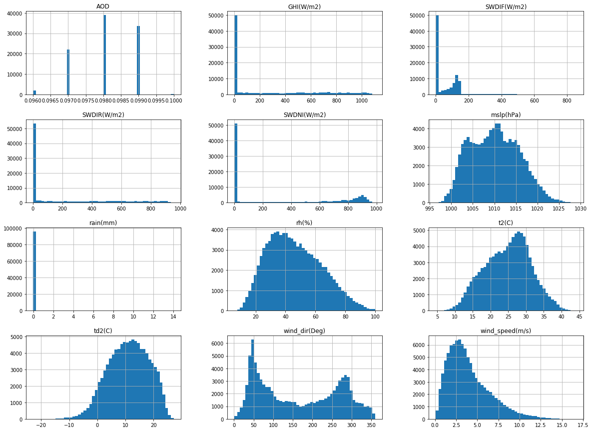
neom_data.describe()
| mslp(hPa) | t2(C) | td2(C) | wind_speed(m/s) | wind_dir(Deg) | rh(%) | GHI(W/m2) | SWDIR(W/m2) | SWDNI(W/m2) | SWDIF(W/m2) | rain(mm) | AOD | |
|---|---|---|---|---|---|---|---|---|---|---|---|---|
| count | 96432.000000 | 96432.000000 | 96432.000000 | 96432.000000 | 96432.000000 | 96432.000000 | 96432.000000 | 96432.000000 | 96432.000000 | 96432.000000 | 96432.000000 | 96432.000000 |
| mean | 1010.110794 | 24.896298 | 11.045605 | 3.991582 | 164.200525 | 46.168410 | 274.757261 | 211.082623 | 331.746291 | 63.674490 | 0.009041 | 0.098086 |
| std | 5.613583 | 6.382410 | 7.153472 | 2.485326 | 102.793404 | 17.874776 | 355.287896 | 296.287340 | 390.765915 | 91.856426 | 0.173081 | 0.000805 |
| min | 996.378000 | 4.571000 | -22.946000 | 0.076000 | 0.672000 | 5.708000 | 0.000000 | 0.000000 | 0.000000 | 0.000000 | -0.037000 | 0.096000 |
| 25% | 1005.539750 | 20.221000 | 5.889750 | 2.152000 | 62.935500 | 32.173000 | 0.000000 | 0.000000 | 0.000000 | 0.000000 | 0.000000 | 0.098000 |
| 50% | 1010.050000 | 25.421000 | 11.324500 | 3.437000 | 149.692000 | 44.200000 | 0.000000 | 0.000000 | 0.000000 | 0.000000 | 0.000000 | 0.098000 |
| 75% | 1014.316000 | 29.466000 | 16.581250 | 5.342000 | 265.977750 | 58.859000 | 579.205250 | 429.275500 | 788.745750 | 121.765250 | 0.000000 | 0.099000 |
| max | 1029.022000 | 44.186000 | 27.196000 | 16.716000 | 359.620000 | 99.929000 | 1103.190000 | 954.562000 | 989.816000 | 856.685000 | 14.038000 | 0.100000 |
_ = neom_data.hist(bins=50, figsize=(20,15))
_hour = (neom_data.index
.hour
.rename("hour"))
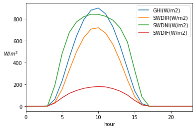
hourly_averages = (neom_data.groupby(_hour)
.mean())
fig, ax = plt.subplots(1, 1)
_targets = ["GHI(W/m2)", "SWDIR(W/m2)", "SWDNI(W/m2)", "SWDIF(W/m2)"]
(hourly_averages.loc[:, _targets]
.plot(ax=ax))
_ = ax.set_ylabel(r"$W/m^2$", rotation="horizontal")
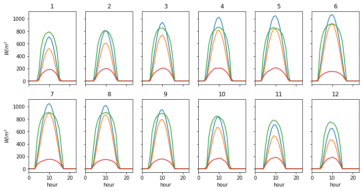
months = (neom_data.index
                   .month
                   .rename("month"))
hours = (neom_data.index
                  .hour
                  .rename("hour"))

hourly_averages_by_month = (neom_data.groupby([months, hours])
                                     .mean())
fig, axes = plt.subplots(2, 6, sharex=True, sharey=True, figsize=(12, 6))

for month in months.unique():
    if month <= 6:
        (hourly_averages_by_month.loc[month, _targets]
                                 .plot(ax=axes[0, month - 1], legend=False))
        _ = axes[0, month - 1].set_title(month)
    else:
        (hourly_averages_by_month.loc[month, _targets]
                                 .plot(ax=axes[1, month - 7], legend=False))
        _ = axes[1, month - 7].set_title(month)

    if month - 1 == 0:
        _ = axes[0, 0].set_ylabel(r"$W/m^2$")
    if month - 7 == 0:
        _ = axes[1, 0].set_ylabel(r"$W/m^2$")
Feature Engineering
_dropped_cols = ["SWDIR(W/m2)", "SWDNI(W/m2)", "SWDIF(W/m2)"]

_year = (neom_data.index
                  .year)
_month = (neom_data.index
                   .month)
_day = (neom_data.index
                 .dayofyear)
_hour = (neom_data.index
                  .hour)

features = (neom_data.drop(_dropped_cols, axis=1, inplace=False)
                     .assign(year=_year, month=_month, day=_day, hour=_hour)
                     .groupby(["year", "month", "day", "hour"])
                     .mean()
                     .unstack(level=["hour"])
                     .reset_index(inplace=False)
                     .sort_index(axis=1)
                     .drop("year", axis=1, inplace=False))
# want to predict the next 24 hours of "solar power"
efficiency_factor = 0.5

# square meters of solar cells required to generate 20 GW (231000 m2 will generate 7mW)
m2_of_solar_cells_required = 660000

target = (features.loc[:, ["GHI(W/m2)"]]
                  .mul(efficiency_factor)
                  .shift(-1)
                  .rename(columns={"GHI(W/m2)": "target(W/m2)"}))
input_data = (features.join(target)
                      .dropna(how="any", inplace=False)
                      .sort_index(axis=1))
input_data
| AOD | ... | wind_speed(m/s) | |||||||||||||||||||
|---|---|---|---|---|---|---|---|---|---|---|---|---|---|---|---|---|---|---|---|---|---|
| hour | 0 | 1 | 2 | 3 | 4 | 5 | 6 | 7 | 8 | 9 | ... | 14 | 15 | 16 | 17 | 18 | 19 | 20 | 21 | 22 | 23 |
| 0 | 0.098 | 0.098 | 0.098 | 0.098 | 0.098 | 0.098 | 0.098 | 0.098 | 0.098 | 0.098 | ... | 1.775 | 0.800 | 0.778 | 0.993 | 1.575 | 1.606 | 2.079 | 2.887 | 3.162 | 3.315 |
| 1 | 0.097 | 0.097 | 0.097 | 0.097 | 0.097 | 0.097 | 0.097 | 0.097 | 0.097 | 0.097 | ... | 2.255 | 1.494 | 0.595 | 0.479 | 2.143 | 3.394 | 3.208 | 2.805 | 3.436 | 4.196 |
| 2 | 0.097 | 0.097 | 0.097 | 0.097 | 0.097 | 0.097 | 0.097 | 0.097 | 0.097 | 0.097 | ... | 3.924 | 1.952 | 1.885 | 1.834 | 3.728 | 5.187 | 5.647 | 6.324 | 7.722 | 8.740 |
| 3 | 0.097 | 0.097 | 0.097 | 0.097 | 0.097 | 0.097 | 0.097 | 0.097 | 0.097 | 0.097 | ... | 5.802 | 4.670 | 3.535 | 4.811 | 5.417 | 5.956 | 7.445 | 8.008 | 8.297 | 8.363 |
| 4 | 0.097 | 0.097 | 0.097 | 0.097 | 0.097 | 0.097 | 0.097 | 0.097 | 0.097 | 0.097 | ... | 6.825 | 5.146 | 4.840 | 3.051 | 7.151 | 4.439 | 3.869 | 6.069 | 9.337 | 10.455 |
| ... | ... | ... | ... | ... | ... | ... | ... | ... | ... | ... | ... | ... | ... | ... | ... | ... | ... | ... | ... | ... | ... |
| 4012 | 0.098 | 0.098 | 0.098 | 0.098 | 0.098 | 0.098 | 0.098 | 0.098 | 0.098 | 0.098 | ... | 2.152 | 0.939 | 0.578 | 0.556 | 0.548 | 1.289 | 2.356 | 3.038 | 3.378 | 4.046 |
| 4013 | 0.097 | 0.097 | 0.097 | 0.097 | 0.097 | 0.097 | 0.097 | 0.097 | 0.097 | 0.097 | ... | 7.200 | 6.153 | 6.734 | 4.120 | 4.700 | 5.639 | 4.562 | 3.876 | 3.941 | 4.160 |
| 4014 | 0.097 | 0.097 | 0.097 | 0.097 | 0.097 | 0.097 | 0.097 | 0.097 | 0.097 | 0.097 | ... | 3.531 | 3.276 | 3.971 | 3.409 | 2.173 | 3.252 | 4.387 | 4.496 | 4.268 | 3.572 |
| 4015 | 0.097 | 0.097 | 0.097 | 0.097 | 0.097 | 0.097 | 0.097 | 0.097 | 0.097 | 0.097 | ... | 4.930 | 4.024 | 3.824 | 3.115 | 1.401 | 2.460 | 3.788 | 4.351 | 4.708 | 4.673 |
| 4016 | 0.097 | 0.097 | 0.097 | 0.097 | 0.097 | 0.097 | 0.097 | 0.097 | 0.097 | 0.097 | ... | 6.060 | 5.376 | 4.654 | 3.102 | 3.931 | 5.463 | 5.687 | 4.491 | 5.557 | 6.213 |
4017 rows × 242 columns
input_data.to_csv("../results/day-ahead/input-data.csv")
Train, Validation, Test Split
# use first eight years for training data...
training_data = input_data.loc[:8 * 365]

# ...next two years for validation data...
validation_data = input_data.loc[8 * 365 + 1:10 * 365 + 1]

# ...and final year for testing data!
testing_data = input_data.loc[10 * 365 + 2:]
training_data.shape
(2921, 242)
validation_data.shape
(731, 242)
testing_data.shape
(365, 242)
Preprocessing the training and validation data
def preprocess_features(df: pd.DataFrame) -> pd.DataFrame:
    _numeric_features = ["GHI(W/m2)",
                         "mslp(hPa)",
                         "rain(mm)",
                         "rh(%)",
                         "t2(C)",
                         "td2(C)",
                         "wind_dir(Deg)",
                         "wind_speed(m/s)"]

    _ordinal_features = ["AOD",
                         "day",
                         "month",
                         "year"]

    standard_scalar = preprocessing.StandardScaler()
    Z0 = standard_scalar.fit_transform(df.loc[:, _numeric_features])

    ordinal_encoder = preprocessing.OrdinalEncoder()
    Z1 = ordinal_encoder.fit_transform(df.loc[:, _ordinal_features])
    transformed_features = np.hstack((Z0, Z1))

    return transformed_features
training_features = training_data.drop("target(W/m2)", axis=1, inplace=False)
training_target = training_data.loc[:, ["target(W/m2)"]]
transformed_training_features = preprocess_features(training_features)

validation_features = validation_data.drop("target(W/m2)", axis=1, inplace=False)
validation_target = validation_data.loc[:, ["target(W/m2)"]]
transformed_validation_features = preprocess_features(validation_features)
Find a few models that seem to work well
Linear Regression
# training a liner regression model
linear_regression = linear_model.LinearRegression()
linear_regression.fit(transformed_training_features, training_target)
LinearRegression(copy_X=True, fit_intercept=True, n_jobs=None, normalize=False)
# measure training error
_predictions = linear_regression.predict(transformed_training_features)
np.sqrt(metrics.mean_squared_error(training_target, _predictions))
16.18214503421171
# measure validation error
_predictions = linear_regression.predict(transformed_validation_features)
np.sqrt(metrics.mean_squared_error(validation_target, _predictions))
18.628289130716887
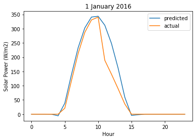
# user requests forecast for 1 January 2016 which we predict using data from 31 December 2015!
user_forecast_request = transformed_training_features[[-1], :]
user_forecast_response = linear_regression.predict(user_forecast_request)[0]
actual_values_response = training_target.values[[-1], :][0]

# this would be rendered in Tableau!
plt.plot(user_forecast_response, label="predicted")
plt.plot(actual_values_response, label="actual")
plt.legend()
plt.title("1 January 2016")
plt.ylabel("Solar Power (W/m2)")
plt.xlabel("Hour")
Text(0.5, 0, 'Hour')
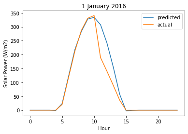
Linear regression is not bad but we an do better!
MultiTask ElasticNet Regression
# training a multi-task elastic net model
_prng = np.random.RandomState(42)
elastic_net = linear_model.MultiTaskElasticNet(random_state=_prng)
elastic_net.fit(transformed_training_features, training_target)
MultiTaskElasticNet(alpha=1.0, copy_X=True, fit_intercept=True, l1_ratio=0.5,
                    max_iter=1000, normalize=False,
                    random_state=<mtrand.RandomState object at 0x1a386672d0>,
                    selection='cyclic', tol=0.0001, warm_start=False)
# measure training error
_predictions = elastic_net.predict(transformed_training_features)
np.sqrt(metrics.mean_squared_error(training_target, _predictions))
18.73221160297961
# measure validation error
_predictions = elastic_net.predict(transformed_validation_features)
np.sqrt(metrics.mean_squared_error(validation_target, _predictions))
17.864005311687215
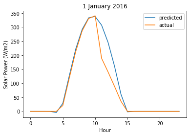
# user requests forecast for 1 January 2016 which we predict using data from 31 December 2015!
user_forecast_request = transformed_training_features[[-1], :]
user_forecast_response = elastic_net.predict(user_forecast_request)[0]
actual_values_response = training_target.values[[-1], :][0]

# this would be rendered in Tableau!
plt.plot(user_forecast_response, label="predicted")
plt.plot(actual_values_response, label="actual")
plt.legend()
plt.title("1 January 2016")
plt.ylabel("Solar Power (W/m2)")
plt.xlabel("Hour")
Text(0.5, 0, 'Hour')
ElasticNet is underfitting.
MultiTask Lasso Regression
# training a multi-task lasso model
_prng = np.random.RandomState(42)
lasso_regression = linear_model.MultiTaskLasso(random_state=_prng)
lasso_regression.fit(transformed_training_features, training_target)
MultiTaskLasso(alpha=1.0, copy_X=True, fit_intercept=True, max_iter=1000,
               normalize=False,
               random_state=<mtrand.RandomState object at 0x1a649d5870>,
               selection='cyclic', tol=0.0001, warm_start=False)
# measure training error
_predictions = lasso_regression.predict(transformed_training_features)
np.sqrt(metrics.mean_squared_error(training_target, _predictions))
17.375320291371146
# measure validation error
_predictions = lasso_regression.predict(transformed_validation_features)
np.sqrt(metrics.mean_squared_error(validation_target, _predictions))
16.14489387119325
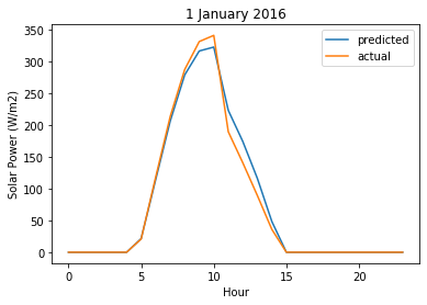
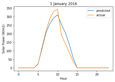
# user requests forecast for 1 January 2016 which we predict using data from 31 December 2015!
user_forecast_request = transformed_training_features[[-1], :]
user_forecast_response = lasso_regression.predict(user_forecast_request)[0]
actual_values_response = training_target.values[[-1], :][0]

# this would be rendered in Tableau!
plt.plot(user_forecast_response, label="predicted")
plt.plot(actual_values_response, label="actual")
plt.legend()
plt.title("1 January 2016")
plt.ylabel("Solar Power (W/m2)")
plt.xlabel("Hour")
Text(0.5, 0, 'Hour')
Lasso Regression is underfitting.
Random Forest Regression
_prng = np.random.RandomState(42)
random_forest_regressor = ensemble.RandomForestRegressor(n_estimators=100, random_state=_prng, n_jobs=2)
random_forest_regressor.fit(transformed_training_features, training_target)
RandomForestRegressor(bootstrap=True, criterion='mse', max_depth=None,
                      max_features='auto', max_leaf_nodes=None,
                      min_impurity_decrease=0.0, min_impurity_split=None,
                      min_samples_leaf=1, min_samples_split=2,
                      min_weight_fraction_leaf=0.0, n_estimators=100, n_jobs=2,
                      oob_score=False,
                      random_state=<mtrand.RandomState object at 0x1284a3558>,
                      verbose=0, warm_start=False)
# measure training error
_predictions = random_forest_regressor.predict(transformed_training_features)
np.sqrt(metrics.mean_squared_error(training_target, _predictions))
6.540426384057337
# measure validation error
_predictions = random_forest_regressor.predict(transformed_validation_features)
np.sqrt(metrics.mean_squared_error(validation_target, _predictions))
17.10706983980618
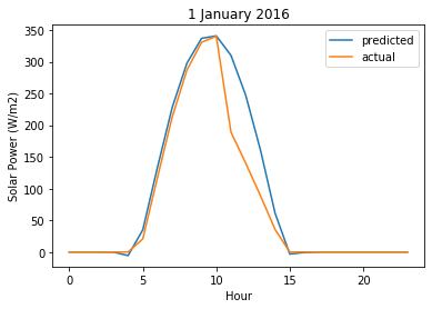
# user requests forecast for 1 January 2016 which we predict using data from 31 December 2015!
user_forecast_request = transformed_training_features[[-1], :]
user_forecast_response = random_forest_regressor.predict(user_forecast_request)[0]
actual_values_response = training_target.values[[-1], :][0]

# this would be rendered in Tableau!
plt.plot(user_forecast_response, label="predicted")
plt.plot(actual_values_response, label="actual")
plt.legend()
plt.title("1 January 2016")
plt.ylabel("Solar Power (W/m2)")
plt.xlabel("Hour")
Text(0.5, 0, 'Hour')
Random Forest with default parameters is over-fitting and needs to be regularized.
Tuning hyper-parameters
from scipy import stats
MultiTask ElasticNet Regression
_prng = np.random.RandomState(42)

_param_distributions = {
    "l1_ratio": stats.uniform(),
    "alpha": stats.lognorm(s=1),
}

elastic_net_randomized_search = model_selection.RandomizedSearchCV(
    elastic_net,
    param_distributions=_param_distributions,
    scoring="neg_mean_squared_error",
    random_state=_prng,
    n_iter=10,
    cv=8,
    n_jobs=2,
    verbose=10
)

elastic_net_randomized_search.fit(transformed_training_features, training_target)
Fitting 8 folds for each of 10 candidates, totalling 80 fits


[Parallel(n_jobs=2)]: Using backend LokyBackend with 2 concurrent workers.
[Parallel(n_jobs=2)]: Done   1 tasks      | elapsed:    7.7s
[Parallel(n_jobs=2)]: Done   4 tasks      | elapsed:   11.2s
[Parallel(n_jobs=2)]: Done   9 tasks      | elapsed:   23.6s
[Parallel(n_jobs=2)]: Done  14 tasks      | elapsed:   36.4s
[Parallel(n_jobs=2)]: Done  21 tasks      | elapsed:  1.4min
[Parallel(n_jobs=2)]: Done  28 tasks      | elapsed:  1.8min
[Parallel(n_jobs=2)]: Done  37 tasks      | elapsed:  2.0min
[Parallel(n_jobs=2)]: Done  46 tasks      | elapsed:  2.1min
[Parallel(n_jobs=2)]: Done  57 tasks      | elapsed:  3.0min
[Parallel(n_jobs=2)]: Done  68 tasks      | elapsed:  3.5min
[Parallel(n_jobs=2)]: Done  80 out of  80 | elapsed:  6.0min finished


RandomizedSearchCV(cv=8, error_score='raise-deprecating',
                   estimator=MultiTaskElasticNet(alpha=1.0, copy_X=True,
                                                 fit_intercept=True,
                                                 l1_ratio=0.5, max_iter=1000,
                                                 normalize=False,
                                                 random_state=<mtrand.RandomState object at 0x1a386672d0>,
                                                 selection='cyclic', tol=0.0001,
                                                 warm_start=False),
                   iid='warn', n_iter=10, n_jobs=2,
                   param_distributions={'alpha': <scipy.stats._distn_infrastructure.rv_frozen object at 0x1a7b2845c0>,
                                        'l1_ratio': <scipy.stats._distn_infrastructure.rv_frozen object at 0x1a7b26f710>},
                   pre_dispatch='2*n_jobs',
                   random_state=<mtrand.RandomState object at 0x12808e318>,
                   refit=True, return_train_score=False,
                   scoring='neg_mean_squared_error', verbose=10)
_ = joblib.dump(elastic_net_randomized_search.best_estimator_,
                "../models/tuned-elasticnet-regression-model.pkl")
elastic_net_randomized_search.best_estimator_
MultiTaskElasticNet(alpha=2.154232968599504, copy_X=True, fit_intercept=True,
                    l1_ratio=0.9699098521619943, max_iter=1000, normalize=False,
                    random_state=<mtrand.RandomState object at 0x1a48e31558>,
                    selection='cyclic', tol=0.0001, warm_start=False)
(-elastic_net_randomized_search.best_score_)**0.5
18.355092813714375
# user requests forecast for 1 January 2016 which we predict using data from 31 December 2015!
user_forecast_request = transformed_training_features[[-1], :]
user_forecast_response = elastic_net_randomized_search.predict(user_forecast_request)[0]
actual_values_response = training_target.values[[-1], :][0]

# this would be rendered in Tableau!
plt.plot(user_forecast_response, label="predicted")
plt.plot(actual_values_response, label="actual")
plt.legend()
plt.title("1 January 2017")
plt.ylabel("Solar Power (W/m2)")
plt.xlabel("Hour")
Text(0.5, 0, 'Hour')
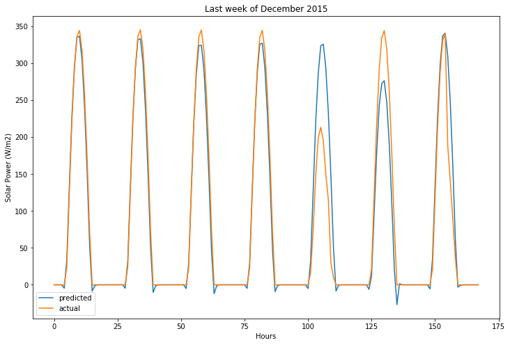
# user requests forecast for last week of 2015
user_forecast_request = transformed_training_features[-7:, :]
user_forecast_response = elastic_net_randomized_search.predict(user_forecast_request)
actual_values_response = training_target.values[-7:, :]

# this would be rendered in Tableau!
fig, ax = plt.subplots(1, 1, figsize=(12, 8))
ax.plot(user_forecast_response.flatten(), label="predicted")
ax.plot(actual_values_response.flatten(), label="actual")
ax.legend()
ax.set_title("Last week of December 2015")
ax.set_ylabel("Solar Power (W/m2)")
ax.set_xlabel("Hours")
Text(0.5, 0, 'Hours')
MultiTask Lasso Regression
_prng = np.random.RandomState(42)

_param_distributions = {
    "alpha": stats.lognorm(s=1),
}

lasso_regression_randomized_search = model_selection.RandomizedSearchCV(
    lasso_regression,
    param_distributions=_param_distributions,
    scoring="neg_mean_squared_error",
    random_state=_prng,
    n_iter=10,
    cv=8,
    n_jobs=2,
    verbose=10
)

lasso_regression_randomized_search.fit(transformed_training_features, training_target)
Fitting 8 folds for each of 10 candidates, totalling 80 fits


[Parallel(n_jobs=2)]: Using backend LokyBackend with 2 concurrent workers.
[Parallel(n_jobs=2)]: Done   1 tasks      | elapsed:    7.0s
[Parallel(n_jobs=2)]: Done   4 tasks      | elapsed:    9.4s
[Parallel(n_jobs=2)]: Done   9 tasks      | elapsed:   16.5s
[Parallel(n_jobs=2)]: Done  14 tasks      | elapsed:   22.5s
[Parallel(n_jobs=2)]: Done  21 tasks      | elapsed:   30.3s
[Parallel(n_jobs=2)]: Done  28 tasks      | elapsed:   38.4s
[Parallel(n_jobs=2)]: Done  37 tasks      | elapsed:   48.6s
[Parallel(n_jobs=2)]: Done  46 tasks      | elapsed:  1.0min
[Parallel(n_jobs=2)]: Done  57 tasks      | elapsed:  1.2min
[Parallel(n_jobs=2)]: Done  68 tasks      | elapsed:  1.5min
[Parallel(n_jobs=2)]: Done  80 out of  80 | elapsed:  1.8min finished


RandomizedSearchCV(cv=8, error_score='raise-deprecating',
                   estimator=MultiTaskLasso(alpha=1.0, copy_X=True,
                                            fit_intercept=True, max_iter=1000,
                                            normalize=False,
                                            random_state=<mtrand.RandomState object at 0x1a649d5870>,
                                            selection='cyclic', tol=0.0001,
                                            warm_start=False),
                   iid='warn', n_iter=10, n_jobs=2,
                   param_distributions={'alpha': <scipy.stats._distn_infrastructure.rv_frozen object at 0x1a7af2b470>},
                   pre_dispatch='2*n_jobs',
                   random_state=<mtrand.RandomState object at 0x1a69473438>,
                   refit=True, return_train_score=False,
                   scoring='neg_mean_squared_error', verbose=10)
_ = joblib.dump(lasso_regression_randomized_search.best_estimator_,
                "../models/tuned-lasso-regression-model.pkl")
(-lasso_regression_randomized_search.best_score_)**0.5
17.956920842745834
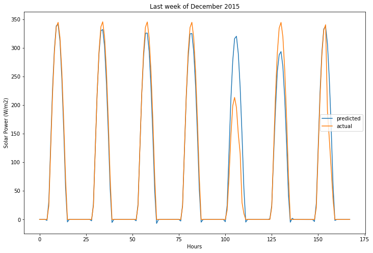
# user requests forecast for last week of 2015
user_forecast_request = transformed_training_features[-7:, :]
user_forecast_response = lasso_regression_randomized_search.predict(user_forecast_request)
actual_values_response = training_target.values[-7:, :]

# this would be rendered in Tableau!
fig, ax = plt.subplots(1, 1, figsize=(12, 8))
ax.plot(user_forecast_response.flatten(), label="predicted")
ax.plot(actual_values_response.flatten(), label="actual")
ax.legend()
ax.set_title("Last week of December 2015")
ax.set_ylabel("Solar Power (W/m2)")
ax.set_xlabel("Hours")
Text(0.5, 0, 'Hours')
Random Forest Regressor
_prng = np.random.RandomState(42)

_param_distributions = {
    "n_estimators": stats.geom(p=0.01),
     "min_samples_split": stats.beta(a=1, b=99),
     "min_samples_leaf": stats.beta(a=1, b=999),
}

_cv = model_selection.TimeSeriesSplit(max_train_size=None, n_splits=5)

random_forest_randomized_search = model_selection.RandomizedSearchCV(
    random_forest_regressor,
    param_distributions=_param_distributions,
    scoring="neg_mean_squared_error",
    random_state=_prng,
    n_iter=10,
    cv=8,
    n_jobs=2,
    verbose=10
)

random_forest_randomized_search.fit(transformed_training_features, training_target)
Fitting 8 folds for each of 10 candidates, totalling 80 fits


[Parallel(n_jobs=2)]: Using backend LokyBackend with 2 concurrent workers.
[Parallel(n_jobs=2)]: Done   1 tasks      | elapsed:   38.3s
[Parallel(n_jobs=2)]: Done   4 tasks      | elapsed:  1.2min
[Parallel(n_jobs=2)]: Done   9 tasks      | elapsed:  2.7min
[Parallel(n_jobs=2)]: Done  14 tasks      | elapsed: 16.6min
[Parallel(n_jobs=2)]: Done  21 tasks      | elapsed: 18.3min
[Parallel(n_jobs=2)]: Done  28 tasks      | elapsed: 18.8min
[Parallel(n_jobs=2)]: Done  37 tasks      | elapsed: 19.2min
[Parallel(n_jobs=2)]: Done  46 tasks      | elapsed: 19.7min
[Parallel(n_jobs=2)]: Done  57 tasks      | elapsed: 20.4min
[Parallel(n_jobs=2)]: Done  68 tasks      | elapsed: 22.3min
[Parallel(n_jobs=2)]: Done  80 out of  80 | elapsed: 24.0min finished


RandomizedSearchCV(cv=8, error_score='raise-deprecating',
                   estimator=RandomForestRegressor(bootstrap=True,
                                                   criterion='mse',
                                                   max_depth=None,
                                                   max_features='auto',
                                                   max_leaf_nodes=None,
                                                   min_impurity_decrease=0.0,
                                                   min_impurity_split=None,
                                                   min_samples_leaf=1,
                                                   min_samples_split=2,
                                                   min_weight_fraction_leaf=0.0,
                                                   n_estimators=100, n_jobs=2,
                                                   oob_score=False,
                                                   random_state=<mt...
                   param_distributions={'min_samples_leaf': <scipy.stats._distn_infrastructure.rv_frozen object at 0x1a5ebd65c0>,
                                        'min_samples_split': <scipy.stats._distn_infrastructure.rv_frozen object at 0x1a625c2a58>,
                                        'n_estimators': <scipy.stats._distn_infrastructure.rv_frozen object at 0x1a5ebd49b0>},
                   pre_dispatch='2*n_jobs',
                   random_state=<mtrand.RandomState object at 0x1a3a76c2d0>,
                   refit=True, return_train_score=False,
                   scoring='neg_mean_squared_error', verbose=10)
_ = joblib.dump(random_forest_randomized_search.best_estimator_,
                "../models/tuned-random-forest-regression-model.pkl")
random_forest_randomized_search.best_estimator_
RandomForestRegressor(bootstrap=True, criterion='mse', max_depth=None,
                      max_features='auto', max_leaf_nodes=None,
                      min_impurity_decrease=0.0, min_impurity_split=None,
                      min_samples_leaf=0.001249828663231378,
                      min_samples_split=0.0019415164208264953,
                      min_weight_fraction_leaf=0.0, n_estimators=75, n_jobs=2,
                      oob_score=False,
                      random_state=<mtrand.RandomState object at 0x125798480>,
                      verbose=0, warm_start=False)
(-random_forest_randomized_search.best_score_)**0.5
17.248545184577317
# user requests forecast for 1 January 2016 which we predict using data from 31 December 2015!
user_forecast_request = transformed_training_features[[-1], :]
user_forecast_response = random_forest_randomized_search.predict(user_forecast_request)[0]
actual_values_response = training_target.values[[-1], :][0]

# this would be rendered in Tableau!
plt.plot(user_forecast_response, label="predicted")
plt.plot(actual_values_response, label="actual")
plt.legend()
plt.title("1 January 2016")
plt.ylabel("Solar Power (W/m2)")
plt.xlabel("Hour")
plt.savefig("../results/img/typical-actual-vs-predicted-solar-power.png")
Assess model performance on testing data
testing_features = testing_data.drop("target(W/m2)", axis=1, inplace=False)
testing_target = testing_data.loc[:, ["target(W/m2)"]]
transformed_testing_features = preprocess_features(testing_features)
elastic_net_predictions = elastic_net_randomized_search.predict(transformed_testing_features)
np.sqrt(metrics.mean_squared_error(testing_target, elastic_net_predictions))
19.76022744338562
lasso_regression_predictions = lasso_regression_randomized_search.predict(transformed_testing_features)
np.sqrt(metrics.mean_squared_error(testing_target, lasso_regression_predictions))
19.73446980783998
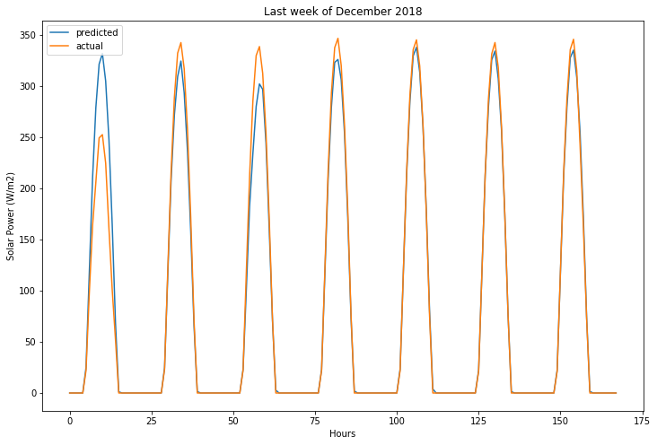
# random forest wins!
random_forest_predictions = random_forest_randomized_search.predict(transformed_testing_features)
np.sqrt(metrics.mean_squared_error(testing_target, random_forest_predictions))
18.977074427410706
# user requests forecast for last week of 2018
user_forecast_request = transformed_testing_features[-7:, :]
user_forecast_response = random_forest_randomized_search.predict(user_forecast_request)
actual_values_response = testing_target.values[-7:, :]

# this would be rendered in Tableau!
fig, ax = plt.subplots(1, 1, figsize=(12, 8))
ax.plot(user_forecast_response.flatten(), label="predicted")
ax.plot(actual_values_response.flatten(), label="actual")
ax.legend()
ax.set_title("Last week of December 2018")
ax.set_ylabel("Solar Power (W/m2)")
ax.set_xlabel("Hours")
Text(0.5, 0, 'Hours')
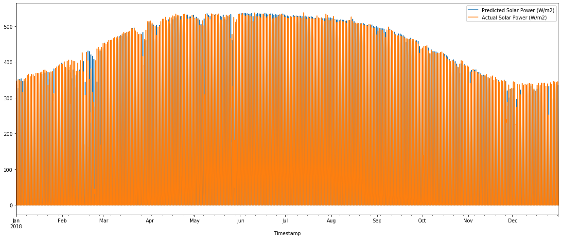
submission = (pd.DataFrame.from_dict({"Timestamp": pd.date_range("2018-01-01", end="2018-12-31 23:00:00", freq="H"),
                                     "Predicted Solar Power (W/m2)": random_forest_predictions.flatten(),
                                     "Actual Solar Power (W/m2)": testing_target.values.flatten()})
                          .set_index("Timestamp", inplace=False))
submission.info()
<class 'pandas.core.frame.DataFrame'>
DatetimeIndex: 8760 entries, 2018-01-01 00:00:00 to 2018-12-31 23:00:00
Data columns (total 2 columns):
Predicted Solar Power (W/m2)    8760 non-null float64
Actual Solar Power (W/m2)       8760 non-null float64
dtypes: float64(2)
memory usage: 205.3 KB
fig, ax = plt.subplots(1, 1, figsize=(20, 8))
_ = submission.plot(ax=ax)
submission.to_csv("../results/actual-vs-predicted-values-for-2018.csv", index=True)
# combine the training and validtion data
combined_training_features = pd.concat([training_features, validation_features])
transformed_combined_training_features = preprocess_features(combined_training_features)
combined_training_target = pd.concat([training_target, validation_target])

# tune a random forest regressor using CV ro avoid overfitting
_prng = np.random.RandomState(42)

_param_distributions = {
    "n_estimators": stats.geom(p=0.01),
     "min_samples_split": stats.beta(a=1, b=99),
     "min_samples_leaf": stats.beta(a=1, b=999),
}

tuned_random_forest_regressor = model_selection.RandomizedSearchCV(
    ensemble.RandomForestRegressor(n_estimators=100, random_state=_prng),
    param_distributions=_param_distributions,
    scoring="neg_mean_squared_error",
    random_state=_prng,
    n_iter=10,
    cv=8,
    n_jobs=2,
    verbose=10
)

tuned_random_forest_regressor.fit(combined_training_features, combined_training_target)
Fitting 8 folds for each of 10 candidates, totalling 80 fits


[Parallel(n_jobs=2)]: Using backend LokyBackend with 2 concurrent workers.
[Parallel(n_jobs=2)]: Done   1 tasks      | elapsed:   59.2s
[Parallel(n_jobs=2)]: Done   4 tasks      | elapsed:  1.9min
[Parallel(n_jobs=2)]: Done   9 tasks      | elapsed:  4.2min
[Parallel(n_jobs=2)]: Done  14 tasks      | elapsed:  5.4min
[Parallel(n_jobs=2)]: Done  21 tasks      | elapsed:  7.6min
[Parallel(n_jobs=2)]: Done  28 tasks      | elapsed:  8.4min
[Parallel(n_jobs=2)]: Done  37 tasks      | elapsed:  9.1min
[Parallel(n_jobs=2)]: Done  46 tasks      | elapsed:  9.6min
[Parallel(n_jobs=2)]: Done  57 tasks      | elapsed: 10.7min
[Parallel(n_jobs=2)]: Done  68 tasks      | elapsed: 13.9min
[Parallel(n_jobs=2)]: Done  80 out of  80 | elapsed: 16.9min finished
/Users/pughdr/Research/junctionx-kaust-2019/env/lib/python3.6/site-packages/sklearn/model_selection/_search.py:813: DeprecationWarning: The default of the `iid` parameter will change from True to False in version 0.22 and will be removed in 0.24. This will change numeric results when test-set sizes are unequal.
  DeprecationWarning)


RandomizedSearchCV(cv=8, error_score='raise-deprecating',
                   estimator=RandomForestRegressor(bootstrap=True,
                                                   criterion='mse',
                                                   max_depth=None,
                                                   max_features='auto',
                                                   max_leaf_nodes=None,
                                                   min_impurity_decrease=0.0,
                                                   min_impurity_split=None,
                                                   min_samples_leaf=1,
                                                   min_samples_split=2,
                                                   min_weight_fraction_leaf=0.0,
                                                   n_estimators=100,
                                                   n_jobs=None, oob_score=False,
                                                   random_state=...
                   param_distributions={'min_samples_leaf': <scipy.stats._distn_infrastructure.rv_frozen object at 0x1a7b7b87f0>,
                                        'min_samples_split': <scipy.stats._distn_infrastructure.rv_frozen object at 0x1a7b7b8f28>,
                                        'n_estimators': <scipy.stats._distn_infrastructure.rv_frozen object at 0x1a7b7b8a20>},
                   pre_dispatch='2*n_jobs',
                   random_state=<mtrand.RandomState object at 0x12a6e0870>,
                   refit=True, return_train_score=False,
                   scoring='neg_mean_squared_error', verbose=10)
tuned_random_forest_regressor.best_estimator_
RandomForestRegressor(bootstrap=True, criterion='mse', max_depth=None,
                      max_features='auto', max_leaf_nodes=None,
                      min_impurity_decrease=0.0, min_impurity_split=None,
                      min_samples_leaf=0.001249828663231378,
                      min_samples_split=0.0019415164208264953,
                      min_weight_fraction_leaf=0.0, n_estimators=75,
                      n_jobs=None, oob_score=False,
                      random_state=<mtrand.RandomState object at 0x12b1bddc8>,
                      verbose=0, warm_start=False)
(-tuned_random_forest_regressor.best_score_)**0.5
17.152712131824202
# user requests forecast for last week of 2018
user_forecast_request = transformed_testing_features[-7:, :]
user_forecast_response = random_forest_randomized_search.predict(user_forecast_request)
actual_values_response = testing_target.values[-7:, :]

# this would be rendered in Tableau!
fig, ax = plt.subplots(1, 1, figsize=(12, 8))
ax.plot(user_forecast_response.flatten(), label="predicted")
ax.plot(actual_values_response.flatten(), label="actual")
ax.legend()
ax.set_title("Last week of December 2018")
ax.set_ylabel("Solar Power (W/m2)")
ax.set_xlabel("Hours")
Text(0.5, 0, 'Hours')

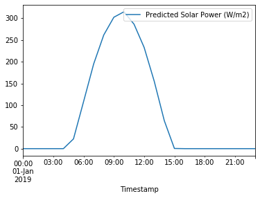
Forecasting the future of solar power at NEOM
Once the model is trained, the model can generate a new forecast for next day’s solar power generation. Once actual values of solar power generation are observed, model can be automatically re-trained and improved. Model can be retrained with weekly, monthly forecast horizons if longer forecasts are required.
incoming_features = features.loc[[4017]]
new_predictions = tuned_random_forest_regressor.predict(incoming_features)[0]
solar_power_forecast = (pd.DataFrame.from_dict({"Timestamp": pd.date_range(start="2019-01-01", end="2019-01-01 23:00:00", freq='H'),
                                                "Predicted Solar Power (W/m2)": new_predictions})
                          .set_index("Timestamp", inplace=False))
_ = solar_power_forecast.plot()
solar_power_forecast.to_csv("../results/solar-power-forecast-20190101.csv")